Stock Market Price Prediction & Forecasting

Here, in this project, we are going to ROCK AND LEARN about how to analyze the data on stock market closing prices in the previous years. We are here to analyze, then predict and forecast the prices in the following years.

We would like to model stock prices correctly, so as a stock buyer we can reasonably decide when to buy stocks and when to sell them to make a profit. This is where time series modelling comes in.

So, let’s get started!

For this stock market prediction first, we need to know what this stock market is actually about.

Stock market analysis is basically a time series analysis. So, the next question that arises is “what is a time series?”

Time series analysis

• A time series is nothing but a sequence of observations taken sequentially in time.
• In other words, it is a set of observations or data points taken at specified time usually at equal intervals and it’s used to predict the future values based on the previous observed values.
• Time series analysis comprises methods for analyzing time series data in order to extract meaningful statistics and other characteristics of the data which unfolds what the data is actually depicting.
• The primary objective of time series analysis is to develop mathematical models that provide plausible descriptions from sample data and bring out stories from the data.

Now we will have a brief idea about “what is forecasting?”

Time Series Forecasting

• Making predictions about the future in the classical statistical handling of time series data is called as forecasting.
• Forecasting involves taking models then fit on historical data and using them to predict future observations

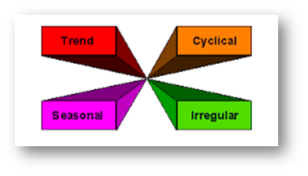
COMPONENTS OF A TIME SERIES

So, let’s start with our analysis.

Stock prices come in several different flavors. They are,

Data Declaration

Open: Opening stock price of the day

Close: Closing stock price of the day

High: Highest stock price of the data

Low: Lowest stock price of the day

Data Types

df.dtypes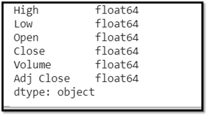

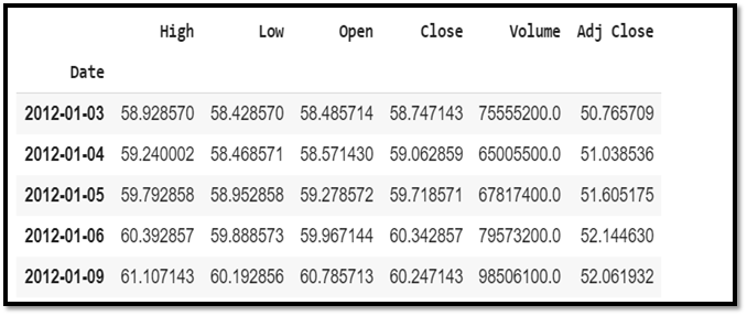
Data Exploration

Here we will print the data you collected in to the Data Frame. We should also make sure that the data is sorted by date, because the order of the data is crucial in time series modelling.

#get the data
df=web.DataReader('AAPL',data_source='yahoo',start='2012-01-01',end='2019-12-17')
#show the data
df.head()

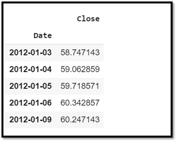
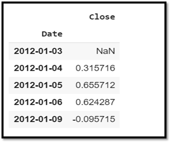
From the whole data frame, in order to analyze and forecast the stock prices we need mainly two columns i.e. “date” and “close”.

From the dataset we need to extract these two columns.

ts=df[['Close']]
ts.head()

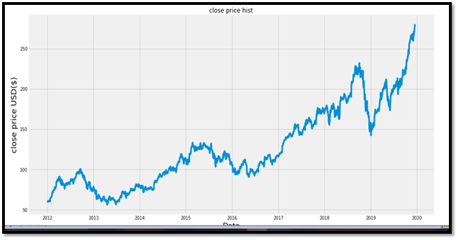
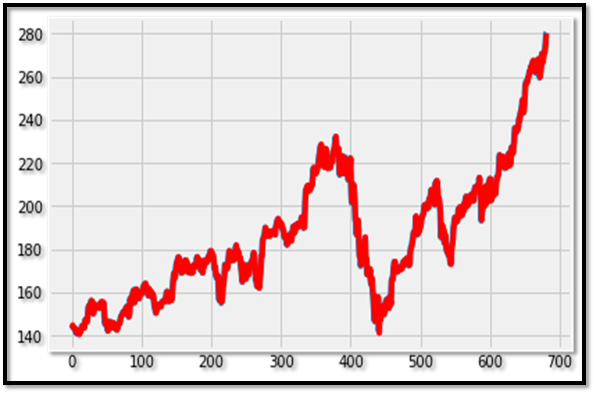
Visualization of data

#visualize closing price history
plot.figure(figsize=(16,8))
plot.title('close price hist')
plot.plot(df['Close'])
plot.xlabel('Date',fontsize=18)
plot.ylabel('close price USD($)',fontsize=18)
plot.show()

Time series forecasting with ARIMA

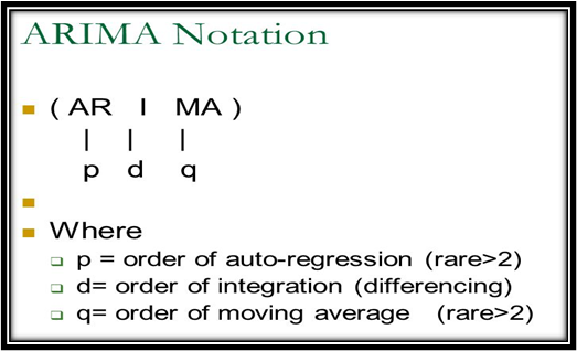
We are going to apply one of the most commonly used method for time-series forecasting, known as ARIMA, which stands for Auto-regressive Integrated Moving Average.

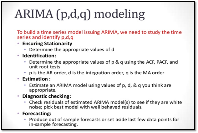
In order to fit the ARIMA model we need to check the stationarity of the model.

The time series data may be of two types:

• Stationary time series
• Non stationary time series

Their graphical representations are as follows:

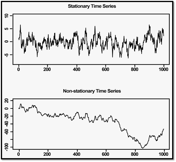
ARIMA model and all the analysis is done on a stationary time series data. So the data needs to be stationarity.

In order to check the stationarity we perform Augmented Dickey-Fuller(ADF)  Test.

We test the following hypothesis:

H_0: the time series data is non stationary.

H_1: the time series data is stationary.

def stationarity(series,mlag=None,lag=None):
  print("RESULT OF ADF TEST")
  res = adfuller(series, maxlag = mlag, autolag = lag)
  output = pd.Series(res[0:4],index = ['Test Statistic', 'p value', 'used lag', 'Number of observations used'])
  for key, value in res[4].items():
     output['Critical Value ' + key] = value
  print(output)

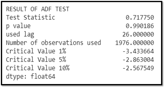
P value > 0.05.

Hence, we fail to reject Ho i.e. the data is non stationary data.

We need to apply differencing method to make it stationary.

Let’s do 1^st order differencing i.e. we take d=1.

ts1=ts.copy()
ts1['Close']=ts1['Close'].diff()

ts1.head()

We need to drop the NA value and after differencing again we need to check stationarity. If again p-value >0.05 then again we will go on differencing untill p< 0.05.

Now once again we check the stationarity after differencing.

So let’s again perform the ADF test.

ts1=ts1.dropna(axis=0)
 stationarity(ts1['Close'])

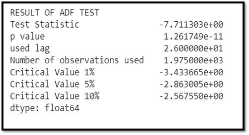
WOW! It’s great.

With one step differencing only the p- value has come soo much less i.e.

p-value < 0.05. Hence we reject Ho i.e. the time series is now stationary. Now  we can perform the model fitting and all that are needed in this stationary time series.

For predicting the values of p, d and q we need to plot auto-correlation function and partial auto-correlation function. From this plotting we will get to know the values of p and q. We already know d=1.

from statsmodels.graphics.tsaplots import plot_acf,plot_pacf
fig = plt.figure(figsize=(16,8))
ax1 = fig.add_subplot(211)
fig = plot_acf(ts["Close"],lags=15,ax=ax1)
plot.title('Autocorrelation Lag=15')
ax2 = fig.add_subplot(212)
fig = plot_pacf(ts["Close"],lags=15,ax=ax2)
plot.title('Partial Autocorrelation Lag=15')
plot.subplots_adjust(left=None, bottom=None, right=None, top=None,
                wspace=None, hspace=0.5)
plot.show()

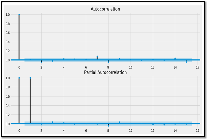
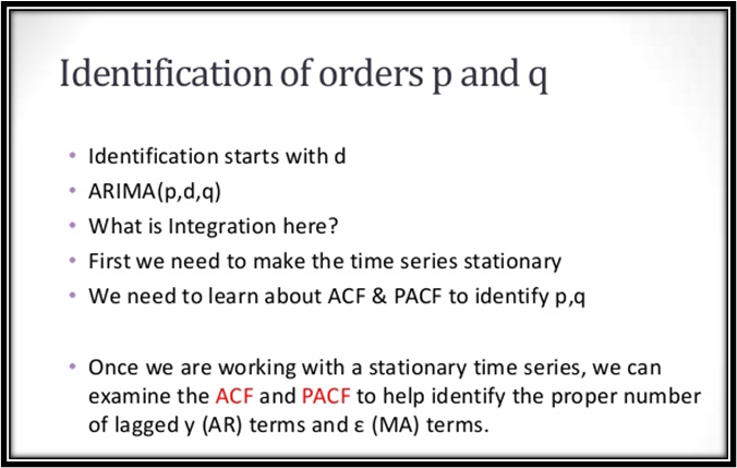
So from the acf and pacf plot we get the values of p,d,q as follows:

p=4

d=1

q=2

Now we are ready to fit the ARIMA(4,1,2) model

timeseries =train
p,d,q = (4,1,2)
arima_mod = ARIMA(timeseries,(p,d,q)).fit()
summary = (arima_mod.summary2(alpha=.05, float_format="%.8f"))
print(summary)

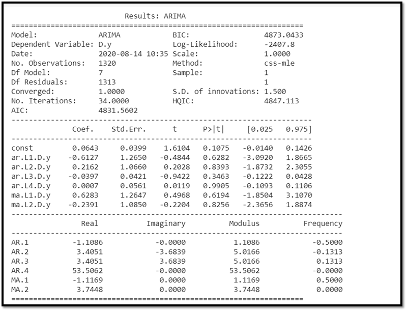
SIGNIFICANCE  OF  AIC

The Akaike Information Critera (AIC) is a widely used measure of a statistical model. It basically quantifies:

 1) the goodness of fit, and

 2) the simplicity/parsimony, of the model into a single statistic. When comparing two models, the one with the lower AIC is generally “better”.

Here AIC= 4831.5602

Now we forecast our model

The Forecasted Model:

plt.plot(test)
plt.plot(predicted1, color='red')
plt.show()

WOW! Its an unexpected forecast. As it can be seen , ARIMA(4,1,2) has fitted so well to this stationary time series data. If we see it very minutely it can be observed that the predicted values are going in hand in hand with the original values. The forecasted graph is almost same as that of the original one.

Hence we can conclude that it has been a very accurate forecast using ARIMA model.

WAIT !                                  

The story is not over yet . There is something more inetersting awaiting for you. We are going to forecast the same using LSTM(Long Short-Term Memory) and this is something very interesting and it is recently introduced to the market. This is basically designed for forecasting stock market price. It is an advanced method unlike ARIMA which is a very basic method that can be used in any stationary time series data. So, are you excited to delve into it? I am sure you must be.

So, let’s get started with our new model LSTM.

LSTM (Long Short-Term Memory)

Here we are using a Keras Long Short-Term Memory (LSTM) Model to Predict Stock Prices. LSTMs are very powerful in sequence prediction problems because they’re able to store past information. This is important in our case because the previous price of a stock is crucial in predicting its future price.

Note: Stock market prices are highly unpredictable and volatile. This means that there are no consistent patterns in the data that allow you to model stock prices over time near-perfectly.

You don’t need the exact stock values of the future, but the stock price movements (that is, if it is going to rise of fall in the near future).

Let’s start with our analysis using LSTM.

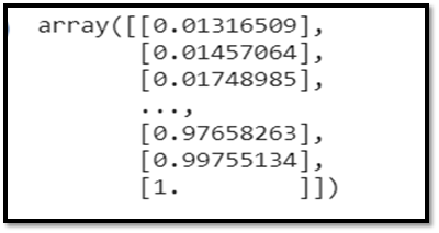
Feature Scaling

 
From previous experience with deep learning models, we know that we have to scale our data for optimal performance. In our case, we’ll use Scikit- Learn’s MinMaxScaler and scale our dataset to numbers between zero and one.

#scale the data
from sklearn.preprocessing import MinMaxScaler
scaler=MinMaxScaler(feature_range=(0,1))
scaled_data=scaler.fit_transform(dataset)
scaled_data

Creating Data with Time-steps

 
LSTMs expect our data to be in a specific format, usually a 3D array. We start by creating data in 60 time steps and converting it into an array using NumPy. Next, we convert the data into a 3D dimension array with X_trainsamples, 60 timestamps, and one feature at each step.

#create the training data set

train_data=scaled_data[0:1603, :]
#split into X-train abd y train
X_train=[]
Y_train=[]
for i in range (60,len(train_data)):
  X_train.append(train_data[i-60:i,0])
  Y_train.append(train_data[i,0])
  if i<=60:
    print(X_train)
    print(Y_train)
    print()

Note: Why LSTM needs 3 dimensional input?

>>> LSTM layer is a recurrent layer, hence it expects 3 D input i.e it wants input dimension , time steps, batch_size.

>>> Empirical evidence shows that LSTM can learn upto 100 time steps ,so feeding larger sequences won’t give you better results.

>>> if your data is not 3 dimensional then reshape it by using ‘.reshape ‘ method. 

Building the LSTM

In order to build the LSTM, we need to import a couple of modules from Keras:

1. Sequential for initializing the neural network
2. Dense for adding a densely connected neural network layer
3. LSTM for adding the Long Short-Term Memory layer
4. Dropout for adding dropout layers that prevent overfitting

#build the model
model=Sequential()
model.add(LSTM(units=50,return_sequences=True,input_shape=(x_train.shape[1],1)))
model.add(LSTM(units=50,return_sequences=False))
model.add(Dense(25))
model.add(Dense(1))

Predicting Future Stock using the Test Set

 First we need to import the test set that we’ll use to make our predictions on.

In order to predict future stock prices we need to do a couple of things after loading in the test set:

1. Merge the training set and the test set on the 0 axis.
2. Set the time step as 60 (as seen previously)
3. Use MinMaxScaler to transform the new dataset
4. Reshape the dataset as done previously

#create testing dataset
#create a new array containing scaled values from index 1543 to 2003
test_data=scaled_data[training_data_len -60:,:]

 x_test=[]
y_test=dataset[training_data_len:, :]
for i in range (60,len(test_data)):
  x_test.append(test_data[i-60:i,0])

 x_test=np.array(x_test)
 x_test=np.reshape(x_test,(x_test.shape[0],x_test.shape[1],1))

After making the predictions we use inverse_transform to get back the stock prices in normal readable format.

#get the models predicted price value
predictions=model.predict(x_test)
predictions=scaler.inverse_transform(predictions)

Significance of RMSE:

The lower the value of the RMSE( Root Mean Square Error) the better is the fit.

Here rmse=0.78255. Hence we can say that the model is well fitted.

#get the rmse
rmse=np.sqrt(np.mean(predictions-y_test)**2)
rmse

Plotting the Results

 
Finally, we use Matplotlib to visualize the result of the predicted stock price and the real stock price.

#plot the results
train=data[:training_data_len]
valid=data[training_data_len:]
valid['Predictions']=predictions

#visualize
plot.figure(figsize=(16,8))
plot.title('model')
plot.xlabel('Date')
plot.ylabel('Close price usd($)')
plot.plot(valid[['Close','Predictions']])
plot.legend()
plot.show()

The forecasted graph:

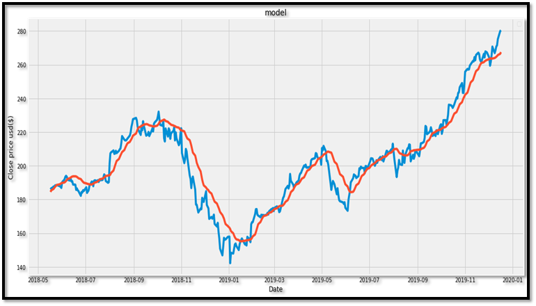
WOW! This is so amazing!

Hence it becomes very clear how LSTM model fits so well in a stock market price forecast.

From the plot we can see that the real stock price went up while our model also predicted that the price of the stock will go up. This clearly shows how powerful LSTMs are for analyzing time series and sequential data.

Advantage of using LSTM over other models:

ARMAs & ARIMAs are particularly simple models which are essentially linear update models plus some noise thrown in. With nonlinear activation functions, neural networks are approximations to nonlinear functions.

RNNs and LSTMs are thus essentially a nonlinear time series model, where the nonlinearity is learned from the data. These will not do well with small amounts of data because it needs to learn the nonlinearity, and training times will be much longer than finding ARMA/ARIMA coefficients. However, with enough data you’ll get an RNN or LSTM which matches the nonlinearities of your real data well, which in term makes its predictions much more accurate than the ARMA / ARIMA.

Conclusion

 
There are a couple of other techniques of predicting stock prices such as moving averages, linear regression, K-Nearest Neighbours, ARIMA and Prophet. These are techniques that one can test on their own and compare their performance with the Keras LSTM.

DISCLAIMER:

Don’t believe blindly on this time series forecasting models on stock price predictions. Unless you are working with financial firm, leverage their infrastructure to do extremely high frequency trading.  Or predict prices with strong cyclical nature.  Stock price is too complicated to be predicted with LSTM unless you do high frequency trading.  Day trading could still be possible with LSTM.  Or the result of LSTM can be treated as a feature to asset ranking system but itself is not sufficient for price prediction.

See the full python notebook here:

---

Written by,

Mentored by,