Predicting diabetes using a Machine Learning model

“The field of study that gives computers the ability to learn without being explicitly programmed.”
– Arthur Samuel (Defined machine learning in 1959)
Machine learning can be used in almost every field nowadays. Using it in the field of medical science can prove to be very beneficial in the improvement of healthcare. Healthcare organizations are leveraging machine learning techniques, to improve delivery of care at reduced cost.
Machine learning is a subset of Artificial Intelligence when combined with Data Mining techniques plays a promising role in the field of prediction.
It is an art and science of giving computers an ability to learn and make decisions from the given data without being explicitly programmed. The way we humans learn from our past experiences.
“The only relevant test of the validity of hypothesis is comparison of prediction with experience”
– Milton Friedman
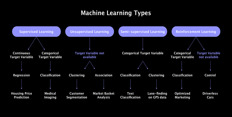
Types of machine learning:
Supervised learning is a learning in which we teach or train the machine using data which is well labelled and expects the output results. That means the input data is already tagged with the correct answer. After that, the machine is provided with a new set of data i.e. test data so that supervised learning algorithm analyses the training data and produces a correct outcome from labelled data.
Unsupervised learning is very much opposite of the supervised learning. It features no labels. Here, an algorithm is only given input data, without corresponding output values, as a training set. There are no correct output values like supervised learning. Instead, algorithms are able to function freely in order to learn more about the data and present interesting findings. In short, Unsupervised learning is data driven and identifies clusters.
Semi-supervised learning the input data that is partially label. It determines correlations between data points then uses the labelled data to mark those data points.
Reinforcement is a machine learning process closely related to Artificial Intelligence. With the aid of some available labelled and incoming data, the machine learns to reinforce and improve itself over time.
Here, we will use a supervised machine learning model to predict whether the patients have diabetes or not.
Diving a bit deeper into the process for carrying out a machine learning model.
There are 7 Steps to create a machine learning model.
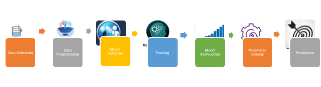
Let’s create our machine learning model to predict whether or not a person has diabetes.
Data Collection & Description
Medical history dataset of people with 7-8 features (Age, Insulin, BMI, Pregnancies, Blood pressure, etc.) to predict whether a person has diabetes or not.
Assuming the hypothesis as,
H_0: The patient does not have diabetes.
H_1: The patient has diabetes.
Where,
Outcome(Y): Dependent variable (1 = person has diabetes/0 = does not have diabetes)
Remaining variables(X) are the independent variables.
Data pre-processing
When it comes to machine learning model, data pre-processing is the first step marking the initiation of the process. Usually, real-world data is incomplete, inconsistent and inaccurate. This is where data processing enters.
We will be solving this problem using Google colab or Jupyter notebook.
The codes for the underlying problem are attached below.
Step1: Importing python libraries and dataset.
Step 2: Checking missing values.
Our dataset contains no missing values. If there exist missing values then it should be either deleted or replaced by mean/median/mode from the data.
Step 3: Encoding the categorical variables.
In python, Sci-kit learn library is used for encoding the variables.
Since, the outcome variable in our dataset are pre-encoded as 0 and 1, while the other variables are quantitative variables.
Hence, encoding the variables is not required here.
Step 4: Splitting the dataset into train and test set.
It is standard in ML to split data into training and test sets. The reason for this is very straightforward: if you try and evaluate your system on data you have trained it on, you are doing something unrealistic. The whole point of a machine learning system is to be able to work with unseen data.
Step 5: Feature Scaling
It is applied to independent variables(X) or features of data. It basically helps to normalise the data within a particular range. Sometimes, it also helps in speeding up the calculations in an algorithm.
There are two types of scaling:
- Standardization

This feature will result having values between -3 and +3 more or less.
2. Normalization

This feature will result having values between 0 and 1. Normalisation is recommended when you have normal distribution in most of your features.
Let’s, check if there is any correlation among the variables in the dataset.
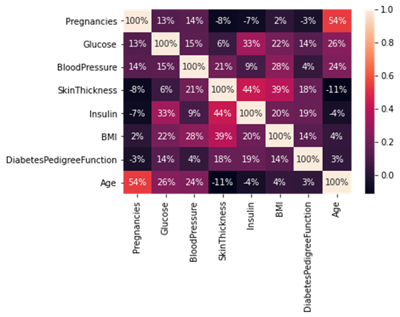
As our dataset contains labelled variables, hence will be solving it using supervised machine learning.
Supervised learning is where you have input variables (x) and an output variable (Y) and you use an algorithm to learn the mapping function from the input to the output.
Y = f(X)
The goal is to approximate the mapping function so well that when you have new input data (x) that you can predict the output variables (Y) for that data.
Supervised learning problems can be further grouped into
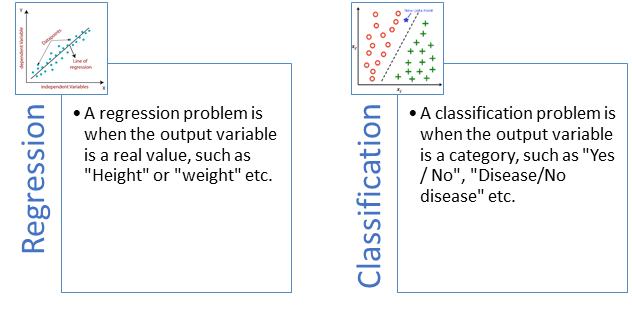
Our problem comes under the classification category, as we have to classify results into whether the patient has diabetes or do not have diabetes.
Model selection
We will be solving the underlying problem using below models because we have a categorical dependent variable.
- Linear Classifier: Logistic Regression
- Decision Tree
- Random Forest
- Neural Network
There are 2 approaches for model selection.
- Structural Risk Minimization (SRM): It is useful when the learning algorithm depends on a parameter that controls the bias-complexity trade-off (such as the degree of the fitted polynomial in the preceding example).
- Validation: The basic idea is to partition the training set into 2 sets. One used for training each of the candidate models, and the second is used for deciding which of them yields the best results.
We will be using 2nd approach in model selection, where the algorithm is applied on train data set and validate to find the accuracy and the model with good accuracy is selected to train for test data. The introduction of a validation dataset allows us to evaluate the model on different data than it was trained on and select the best model architecture, while still holding out a subset of the data for the final evaluation at the end of our model development.
def models(x_train,y_train):
  #logistic
  from sklearn.linear_model import LogisticRegression
  log=LogisticRegression(random_state=0)
  log.fit(x_train,y_train)

  #Decision tree
  from sklearn.tree import DecisionTreeClassifier
  tree=DecisionTreeClassifier(criterion='entropy',random_state=0)
  tree.fit(x_train,y_train)

  #rf
  from sklearn.ensemble import RandomForestClassifier
  rf= RandomForestClassifier(n_estimators=10,criterion='entropy',random_state=0)
  rf.fit(x_train,y_train)

  #print the model accuracy
  print('[0] Logistic accuracy:',log.score(x_train,y_train))
  print('[1] Decision Tree accuracy:',tree.score(x_train,y_train))
  print('[2] random forest accuracy:',rf.score(x_train,y_train))
  return log,tree,rf
Output:
[0] Logistic accuracy: 0.762214983713355
[1] Decision Tree accuracy: 1.0
[2] random forest accuracy: 0.9820846905537459
Here, we have used Logistic regression model for further predictions as random forest and decision trees models shows overfitting. A model with accuracy between 75 to 90 is considered best. While any accuracy above or below the given is range is either overfitting or underfitting model.
Training and model evaluation
We will train our model for Logistic regression.
Logistic regression also called as logit regression or even logit model. It is used to describe the relationship between one dichotomous dependent attribute (Y) and one or more nominal independent variables (X).
Logistic regression is a simple form of a neural network.
In this step, we will use our data to incrementally improve our model’s ability to predict whether or not a person has diabetes.
from sklearn.linear_model import LogisticRegression log=LogisticRegression(random_state=0)
log.fit(x_train,y_train)
Model evaluation is required to quantify the performance of model. Model classification metrics is used in python to check the model’s performance. We will be using classification accuracy, confusion matrix and F score to evaluate the model.
Where,
- Classification accuracy(accuracy_score) computes subset accuracy: the set of labels predicted for a sample must exactly match the corresponding set of labels in y_true.
- Confusion matrix is a summary of prediction results on a classification problem. The number of correct and incorrect predictions are summarized with count values and broken down by each class.
- F1 score can be interpreted as a weighted average of the precision and recall, where an F1 score reaches its best value at 1 and worst score at 0. The relative contribution of precision and recall to the F1 score are equal. The formula for the F1 score is:
F1 = 2 * (precision * recall) / (precision + recall)
In the multi-class and multi-label case, this is the average of the F1 score of each class with weighting depending on the average parameter.
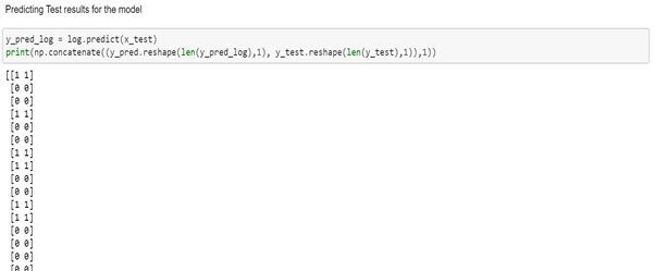
Predictions of Logistic model
The predicted values of the logistic regression model are shown below.
Here, y_pred_log are the predicted values of the logistic regression model and y_test are the values of the test data set. We can find that the predicted values and test values are almost same.
Now, we will continue to build our model with neural networks.
Neural networks can be seen in most places where AI has made steps within the healthcare industry. Hence, we will further build our model using neural network.
Neural Network model
A neural network is a series of algorithms that endeavours to recognize underlying relationships in a set of data through a process that mimics the way the human brain operates.
Architecture of Neural network
Neural network has 3 layers.
- Input Layer
- Hidden layer
- Output layer
The information is passed on through the input layer to hidden and output layers.
How do Neural networks work?
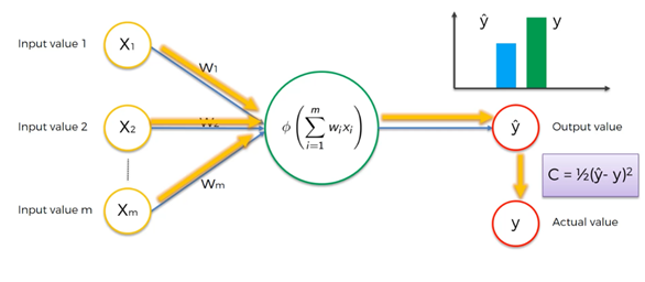
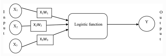
Where,
X1, X2, X3, …Xm: independent variables
W1, W2, W3, ……. Wm: weights
Ø: Activation function
C: Cost function
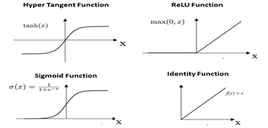
- Activation function (Ø)
Activation function decides, whether a neuron should be activated or not by calculating weighted sum and further adding bias with it. The purpose of the activation function is to introduce non-linearity into the output of a neuron.
There are 3 types of activation function.
- Binary Step Function
- Linear Activation Function
- Non-Linear Activation Functions
We will use Non-Linear Activation Functions in our model named sigmoid and relu.
- Cost function
A cost function is a measure of how wrong the model is in terms of its ability to estimate the relationship between X and y. This is typically expressed as a difference or distance between the predicted value and the actual value.

neural_model=Sequential()
neural_model.add(Dense(16,input_dim=8,activation='relu'))
neural_model.add(Dropout(0.2))
neural_model.add(Dense(32,activation='relu'))
neural_model.add(Dropout(0.2))
neural_model.add(Dense(64,activation='relu'))
neural_model.add(Dropout(0.2))
neural_model.add(Dense(1,activation='sigmoid'))
In the above codes, sequential is used to initialize the neural network and relu is an input layer and the first hidden layer with dimension 8 (independent variables) with 16 units, relu with 32 units is the second hidden layer and relu with 64 units is the third hidden layer. Sigmoid is the output layer of the model.
In the example above, we have added a new Dropout layer between the input (or visible layer) and the first hidden layer. The dropout rate is set to 20%, meaning one in 8 inputs will be randomly excluded from each update cycle.
neural_model.compile(optimizer='adam',loss='binary_crossentropy',metrics=['accuracy'])Stochastic gradient descent termed as adam is the most commonly used optimizer while building a neural network model.
Dependent variable is categorical with two classification values 0 and 1. Hence, binary_crossentropy loss function is used.
Steps for training the Stochastic gradient descent neural network model:
Step1: Randomly initialise the weights to small numbers close to 0 (but not 0).
Step2: Input the first observation of our dataset in the input layer, each feature in one function in one input node.
Step3: Forward-Propagation: from left to right, the neurons are activated in a way that the impact of each neuron’s activation is limited by the weights. Propagate the activation until getting the predicted result y.
Step 4: Compare the predicted result to the actual result. Measure the generated error.
Step5: Back-Propagation: from right to left, the error is back-propagated. Update the weights according to how much they are responsible for the error. The learning rate decides by how much we update the weights.
Step6: Repeat step 1 to 5 and update weight after each/batch of observation.
Step7: When the whole training set passed through the neural network, that makes an epoch. Redo more epochs.
Predictions of Neural Network model
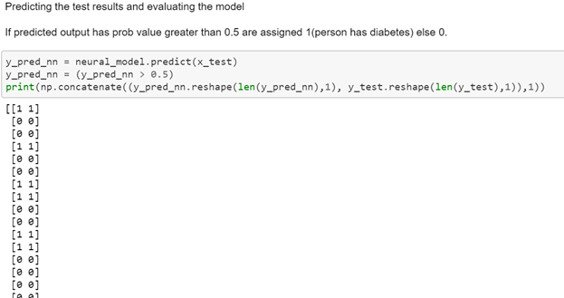
Evaluating the model by confusion matrix and accuracy score.
cm = confusion_matrix(y_test, y_pred_nn)
print(cm)
accuracy_score(y_test, y_pred_nn)
Output:
[[95 12]
 [17 30]]
0.8116883116883117


Accuracy score of both the models on the test data.
Accuracy score of logistic regression model: 0.7987012987012987
Accuracy score of Neural Network model: 0.8116883116883117
Conclusion
Neural networks are one of the most beautiful programming paradigms ever invented. In the conventional approach to programming, we tell the computer what to do and break big problems up into many small, precisely defined tasks that the computer can easily perform. In contrast, we don’t tell the computer how to solve our problems for a neural network. Instead, it learns from observational data and figures out its own solution to the problem.
You can find the code of this work on my GitHub repo
Nimisha Jadhav
Mentored by

wonderful post
I have to show some thanks to this writer just for rescuing me from this circumstance. After looking out through the world-wide-web and obtaining methods which are not pleasant, I figured my entire life was well over. Existing devoid of the strategies to the problems you have solved all through your blog post is a serious case, and those that would have negatively damaged my entire career if I had not discovered the website. Your own understanding and kindness in dealing with all areas was helpful. I don’t know what I would’ve done if I hadn’t encountered such a subject like this. I am able to at this time look forward to my future. Thanks for your time so much for your high quality and sensible guide. I won’t hesitate to recommend your site to any person who desires guide on this area.
My husband and i have been so satisfied when Michael managed to finish up his homework with the precious recommendations he discovered from your own blog. It is now and again perplexing to simply be offering strategies which often others have been selling. Therefore we fully grasp we have got the writer to be grateful to because of that. Most of the explanations you made, the simple website navigation, the relationships you make it possible to create – it’s got mostly awesome, and it’s helping our son and our family know that this situation is interesting, which is certainly rather essential. Many thanks for the whole lot!