Detection of Fake news via NLP

“Disinformation is duping.

Misinformation is tricking.”

― Toba Beta, Master of Stupidity

In today’s era it is difficult to say whether the news published is real or fake.Since fake news attempts to spread false claims in news content, the most straightforward means of detecting it is to check the truthfulness of major claims in a news article to decide the news veracity.

        Since a large proportion of the population uses social media for updating themselves with news, delivering accurate and altruistic information to them is of utmost importance. The news content is diverse in terms of styles, the subject in which it is written, it becomes essential to bring an efficient system for its detection. 

 The purpose of the work is to come up with a solution that can be utilized by users to detectand filter out sites containing false and misleading information.

          So here in this project we will use simple and carefully selected features of the title and news to accurately identify fake news and learn how to detect Fake News.

Natural Language Processing

NLP is a field in machine learning with the ability of a computer to understand, analyze, manipulate, and potentially generate human language.

NLP makes it possible for humans to talk to machines:” This branch of Artificial Intelligence enables computers to understand, interpret, and manipulate human language. Like machine learning or deep learning, NLP is a subset of Artificial Intelligence (AI) where AI is a branch of computer science that emphasises development of intelligence machines, thinking and working like humans. Example: speech recognition, problem-solving, learning and planning.

Let’s get started with our analysis:

The data we are using is Fake News dataset , to proceed with any analysis firstly we need to explore the data .

DATA EXPLORATION

The libraries used here are

import pandas as pd
import numpy as np

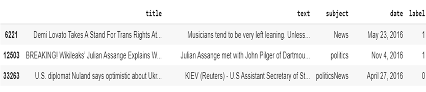
     Here the data is already in Data Frame format . The column ‘label’  tells us whether the data in the row is fake or true which is our output. Since our data is in two different files we will be using the command ‘concat’ and join the two tables , axis = 0 tells us that we wan to join the tables row-wise.

data[ ‘ label ’ ] = 1 is for fake news

data[ ‘ label ’ ] = 0 is for true news

data=pd.concat([fake,true],axis=0,ignore_index=True)
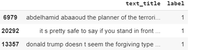
data.sample(5)

data.shape

(44898, 5)

Shape of the dataset :

Rows = 44898   Columns = 5

The next step is to check whether there are any null values in the data

data.isnull().sum()

Output :

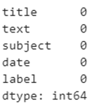
We can see there are no null values.

If there is any  null value, we will use the following command to remove it.

data.dropna()

We will be combining columns ‘ text ‘ and ‘ title ’

This combining should be done only when we know that the content is relevant to the title.

data['text_title']=data['text'] + " " + data['title']
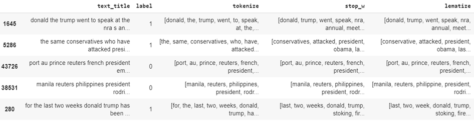
data.sample(5)

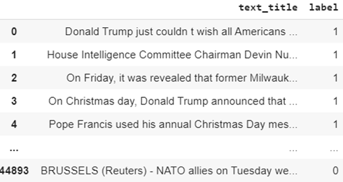
Since in detecting fake news we only need two columns we are going to make a new DataFrame containing only the required columns.

data_new=data[['text_title','label']]
data_new.reset_index()
data_new

PREPROCESSING

CLEANING DATA

data_new['text_title']=data_new['text_title'].str.replace('[^a-zA-Z]',' ')
data_new['text_title']=[word.lower() for word in data_new['text_title']]
data_new.sample(5)

The  first command removes all the punctuations and numbers replacing it with space.

The second command lowers all the  Capital letters.

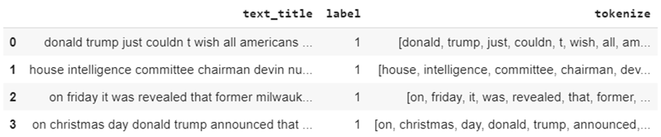
TOKENIZATION

        Tokenization is a task of breaking text into words or sentences. Before processing a natural language, we need to identify the words that constitute a string of characters. That’s why tokenization is the most basic step to proceed with NLP (text data). This is important because the meaning of the text could easily be interpreted by analyzing the words present in the text.

Tokenization using NLTK

        NLTK, short for Natural Language ToolKit, is a library written in Python for symbolic and statistical Natural Language Processing. Some types of NLTK tokenizers are mentioned here:

• Tweet Tokenizer : One of the most interesting features of TweetTokenizer is parameter of  ‘ reduce_len ‘ parameters which is to replace repeated character sequences of length 3 or greater with sequences of length 3 and parameter of  ‘ remove_handles ‘  which is to remove Twitter username handles from text.

• White Space tokenizer : We are able to extract the tokens from string of words or sentences without whitespaces, new line and tabs.

Word Punctuation Tokenizer : Tokenizing and removing all punctuation marks from a sentence removes all punctuation marks from each word.

import nltk
nltk.download('punkt')
from nltk.tokenize import WhitespaceTokenizer
data_new['tokenize']=data_new['text_title'].apply(nltk.tokenize.WhitespaceTokenizer().tokenize)

STOPWORDS removal

Stop words are words that are filtered out before or after the natural language data (text) are processed. While “stop words” typically refers to the most common words in a language, all-natural language processing tools don’t use a single universal list of stop words

nltk.download('stopwords')
from nltk.corpus import stopwords
stop=set(stopwords.words('english'))
data_new['stop_w']=data_new['tokenize'].apply(lambda x:[w for w in x if not w in stop])

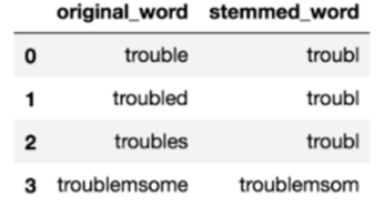
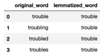
LEMMATIZATION

Lemmatization is the process of grouping together the different  forms of a word so they can be analysed as a single item or considered in a single group. It links words with similar meaning to one word.  The difference is that ‘ stem ’ might not be an actual word whereas, lemma is an actual language word.

            Text preprocessing includes Stemming and Lemmatization we will be using Lemmatization as it is more optimum for use.

nltk.download('wordnet')
from nltk.stem.wordnet import WordNetLemmatizer
def lema_words(text):
  wnl=WordNetLemmatizer()
  return[wnl.lemmatize(w) for w in text]

data_new['lematize']=data_new['stop_w'].apply(lema_words)  
data_new.sample(5)

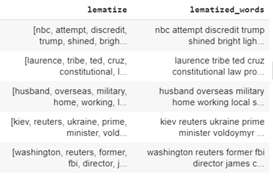
Since we cannot further proceed with the ‘ lematize ‘ column as it is in the list format. We will use the below command to transform it into a continuous format.

data_new['lematized_words']=0
for i in range(0,len(data_new)):
  data_new['lematized_words'][i] = ' '.join(data_new['lematize'][i])

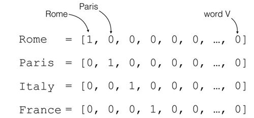
VECTORIZATION

Word vectorization is a methodology in NLP to map words or phrases from vocabulary to a corresponding vector of real numbers which is used to find word predictions, word similarities. The process of converting words into numbers is called Vectorization.

from sklearn.feature_extraction.text import CountVectorizer,TfidfTransformer
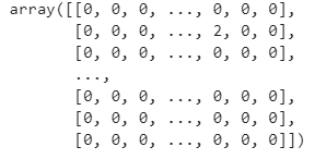
cv=CountVectorizer(max_features=1000)
vect=cv.fit_transform(data_new.lematized_words).toarray()
vect

Tf means term-frequency while tf-idf means term-frequency times inverse document-frequency.The goal of using tf-idf instead of the raw frequencies of occurrence of a token in a given document is to scale down the impact of tokens that occur very frequently in a given corpus and that are hence empirically less informative than features that occur in a small fraction of the training corpus.

tfidf_transformer=TfidfTransformer(use_idf=True)
tfidf_array=tfidf_transformer.fit_transform(vect).toarray()
tfidf_array

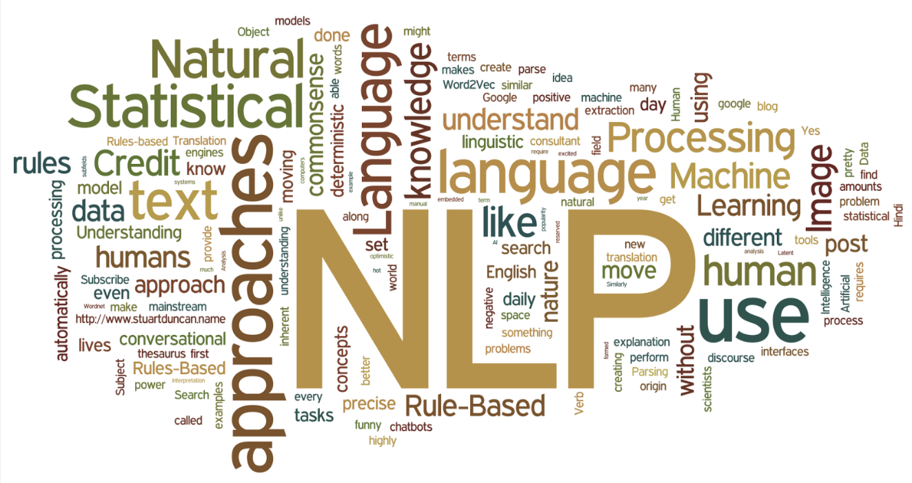
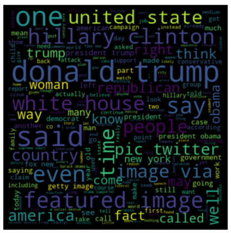
WORDCLOUD

WordCloud is a technique to show which words are the most frequent among the given text.

We will be doing WordCloud for Fake News

import matplotlib.pyplot as plt
from wordcloud import WordCloud
fake_cloud=''.join(data_new[data_new.label==1]['lematized_words'])
fake_cloud=WordCloud(width=520, height=520).generate(fake_cloud)
plt.figure(figsize=(5,5),facecolor='k')
plt.imshow(fake_cloud)
plt.axis('off')
plt.tight_layout(pad=0)
plt.show()

Similarly, WordCloud could be done for True News.

FITTING THE MODEL

The initial step is to split the array in training and testing

data_x=tfidf_array
data_y=data_new['label']

#splitting data into train and test
from sklearn.model_selection import train_test_split
xtrain,xtest,ytrain,ytest=train_test_split(tfidf_array,data_y,test_size=0.3,random_state=0)

Here are different models that we are going to train

1. Random Forest

      The Random Forest Classifier is a set of decision trees from randomly selected subset of training set. It aggregates the votes from different decision trees to decide the final class of the test object. In random forest we use multiple random decision trees for a better accuracy.

from sklearn.ensemble import  RandomForestClassifier
rfc=RandomForestClassifier(random_state=0)
rfc.fit(xtrain,ytrain)
ypred=rfc.predict(xtest)

Now, after fitting the model we will check for accuracy and other results.

from sklearn.metrics import classification_report,confusion_matrix,accuracy_score
#accuracy of the model
accuracy= round((accuracy_score(ytest,ypred)*100),2)
print("Accuracy is {}".format(accuracy))
Accuracy is 99.76
#confusion matrix
print("confusion_matrix:")
LABEL=['0','1']
import matplotlib.pyplot as plt
import seaborn as sns
conf=confusion_matrix(ytest,ypred)
plt.figure(figsize=(5,5))
sns.heatmap(conf,xticklabels=LABEL,yticklabels=LABEL,annot=True,
fmt='d')
plt.show()

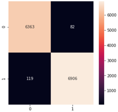
Here, the confusion matrix tells us that –

• 13 which is true news is wrongly predicted as fake news.
• 19 which is fake news is wrongly predicted as true news.
• 6432 is true news is also predicted as true news.
• 7006 is fake news is also predicted as fake news.

2. Logistic Regression

         Logistic regression is most commonly used when the data has binary output, so when it belongs to one class or another, or is either a 0 or 1.

from sklearn.linear_model import LogisticRegression
lr=LogisticRegression(random_state=0)
lr.fit(xtrain,ytrain)
y_pred=lr.predict(xtest)

Let’s check for accuracy and other results ,

from sklearn.metrics import classification_report,confusion_matrix,accuracy_score
#accuracy of the model
accuracy_lr= round((accuracy_score(ytest,y_pred)*100),2)
print("Accuracy is {}".format(accuracy_lr))

Accuracy is 98.51

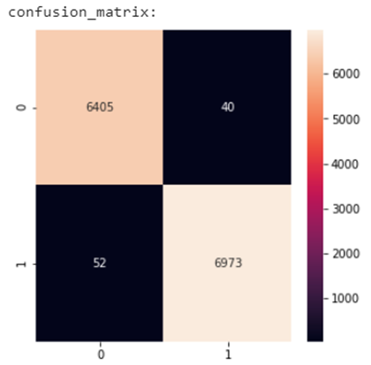
#confusion matrix
print("confusion_matrix:")
LABEL=['0','1']
import matplotlib.pyplot as plt
import seaborn as sns
conf_lr=confusion_matrix(ytest,y_pred)
plt.figure(figsize=(5,5))
sns.heatmap(conf_lr,xticklabels=LABEL,yticklabels=LABEL,annot=True,fmt='d')

3. Decision Tree

      Decision trees provide an effective method of Decision Making because they:

• Clearly lay out the problem so that all options can be challenged.
• Allow us to analyze fully the possible consequences of a decision.
• Provide a framework to quantify the values of outcomes and the probabilities of achieving them.

from sklearn.tree import DecisionTreeClassifier
dcf=DecisionTreeClassifier(random_state=0)
dcf.fit(xtrain,ytrain)
ypred_dcf=dcf.predict(xtest)
accuracy_dcf=round((accuracy_score(ytest,ypred_dcf)*100),2)
print("Accuracy score of decison tree is {}".format(accuracy_dcf))

Accuracy score of decison tree is 99.54

4. Support Vector Machine

Support Vector Machine (SVM) is a supervised machine learning algorithm capable of performing classification, regression and even outlier detection. The linear SVM classifier works by drawing a straight line between two classes .

from sklearn.svm import SVC
svm=SVC(kernel='rbf')
svm.fit(xtrain,ytrain)
y_pred_svm=svm.predict(xtest)

Let’s check for accuracy and other results

accuracy_svm=round((accuracy_score(ytest,y_pred_svm)*100),2)        
print("Accuracy of SVM is {}".format(accuracy_svm))
Accuracy of SVM is 99.32
#confusion matrix
print("confusion_matrix:")
LABEL=['0','1']
import matplotlib.pyplot as plt
import seaborn as sns
conf_lr=confusion_matrix(ytest,y_pred_svm)
plt.figure(figsize=(5,5))
sns.heatmap(conf_lr,xticklabels=LABEL,yticklabels=LABEL,annot=True,fmt='d')
plt.show()

5. Neural Network

      While a Machine Learning model makes decisions according to what it has learned from the data, a Neural Network arranges algorithms in a fashion that it can make accurate decisions by itself. 

input_dim=xtrain.shape[1]

from keras.layers import Dense,Dropout
from keras.models import Sequential

model=Sequential()
model.add(Dense(50,input_dim=input_dim,activation='relu'))
model.add(Dropout(0.3))
model.add(Dense(20,activation='relu'))
model.add(Dropout(0.3))
model.add(Dense(1,activation='sigmoid'))

model.compile(loss='binary_crossentropy',optimizer='adam',
metrics=['accuracy'])

#history records training metrics for each epoch. 
history=model.fit(xtrain,ytrain,batch_size=20,epochs=10,verbose=1,validation_data=(xtest,ytest))
print(history.history.keys())
 

#testing data
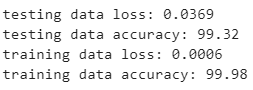
loss_NN,accuracy_NN=model.evaluate(xtest,ytest,verbose=False)
print("testing data loss: {:.4f}".format(loss_NN))
print("testing data accuracy: {:.2f}".format((accuracy_NN)*100))

#training data
loss1,accuracy1=model.evaluate(xtrain,ytrain,verbose=False)
print("training data loss: {:.4f}".format(loss1))
print("training data accuracy: {:.2f}".format((accuracy1)*100))

Output:

REPRESENTATION OF TRAINING NEURAL NETWORK

plt.figure(figsize=(6,5))
plt.plot(history.history['accuracy'])
plt.plot(history.history['val_accuracy'])
plt.title('model accuracy')
plt.ylabel('accuracy')
plt.xlabel('epoch')
plt.legend(['train', 'test'])
plt.show()

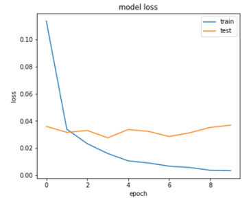
# summarize history for loss
#plt.subplot(1,2,2)
plt.figure(figsize=(6,5))
plt.plot(history.history['loss'])
plt.plot(history.history['val_loss'])
plt.title('model loss')
plt.ylabel('loss')
plt.xlabel('epoch')
plt.legend(['train', 'test'])
plt.show()

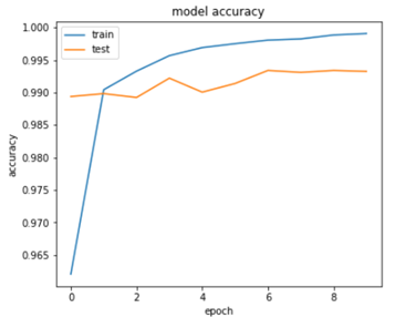
In the first diagram we can see accuracy of training and testing data increasing.

In the second diagram the loss of training and testing data reducing.

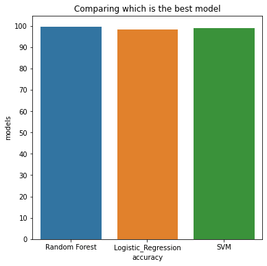
COMPARING DIFFERENT MODELS TO SEE WHICH IS BETTER

COMPARING DIFFERENT MODELS TO SEE WHICH IS BETTER
model=['Random Forest','Logistic_Regression','SVM','Decision_Tree']
acc=[accuracy,accuracy_lr,accuracy_svm,accuracy_dcf]
plt.figure(figsize=(6,6))
plt.yticks(np.arange(0,110,10))
sns.set_style('white')
sns.barplot(model,acc)
plt.title('Comparing which is the best model')
plt.xlabel('accuracy')
plt.ylabel('models')
plt.show()

EXPLAINING WITH LIME

• The first step is to  create a pipeline.

cv=Vectorizer

rfc=Random Forest Classifier

from lime import lime_text
from sklearn.pipeline import make_pipeline
c=make_pipeline(cv,rfc)

• Now we create an explainer object where our ‘ class_names ‘ is defined as [0,1].

a=[0,1]
from lime.lime_text import LimeTextExplainer
explainer = LimeTextExplainer(class_names=a)

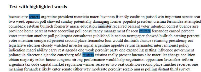
• The last step is to create an explanation with  at most 7 features.

import random
idx=random.randint(0,len(data_new))
exp=explainer.explain_instance(data_new['lematized_words'][idx],c.predict_proba,num_features=7)
print("document_id: %d" % idx)
print("probability_fake_news = " , c.predict_proba([data_new['lematized_words'][idx]])[0,1])
print(" True class : %s" % data_new.label[idx])

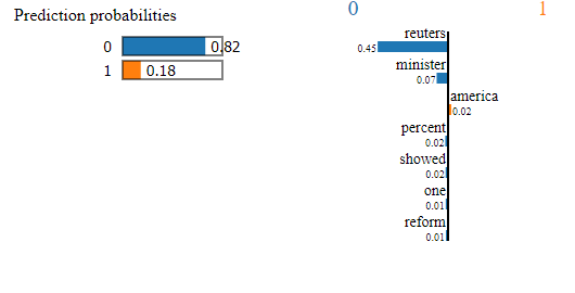
We can see the accuracy of models to be approximately 98% – 99% since the data we are using here is manually labelled ,in general it is overfitting but with LIME we see that it is not overfitting the data. The testing data is also manually labelled. If we go to predict real world’s news then we can see that model’s accuracy drastically reduces to 65% – 70%.

---

Project by,

Mentored by,