Introduction to Time Series Analysis and Forecasting — I

Time series analysis comprises methods for analyzing time series data in order to extract meaningful statistics and other characteristics of the data. Time series forecasting is the use of a model to predict future values .
In this tutorial we are going to discuss about the results and the theory behind them based on ‘Predict Future Sales’ data set .
Note: The downloadable link of the data set will be given below. I will request to download that and try to predict in your own way.
Data set Description:
we have:
- date — every date of items sold
- date_block_num — this number given to every month
- shop_id — unique number of every shop
- item_id — unique number of every item
- item_price — price of every item
- item_cnt_day — number of items sold on a particular day
Packages we need:
import warnings
import itertools
import numpy as np
import matplotlib.pyplot as plt
warnings.filterwarnings("ignore")
plt.style.use('fivethirtyeight')
import pandas as pd
import statsmodels.api as sm
from statsmodels.tsa.arima_model import ARIMA
from pandas.plotting import autocorrelation_plot
from statsmodels.tsa.stattools import adfuller, acf, pacf,arma_order_select_ic
import matplotlibmatplotlib.rcParams['axes.labelsize'] = 14
matplotlib.rcParams['xtick.labelsize'] = 12
matplotlib.rcParams['ytick.labelsize'] = 12
matplotlib.rcParams['text.color'] = 'k'
read the data:
df=pd.read_csv('sales_train.csv')
df.head()
Data types:
date               object
date_block_num      int64
shop_id             int64
item_id             int64
item_price        float64
item_cnt_day      float64
dtype: object
Now we have to convert “date” object to string (YYYY-MM-DD)
import datetime
df['date']=pd.to_datetime(df.date)
Visualizing the time series data:
ts=df.groupby(["date_block_num"])["item_cnt_day"].sum()
ts.astype('float')
plt.figure(figsize=(16,8))
plt.title('Total Sales of the company')
plt.xlabel('Time')
plt.ylabel('Sales')
plt.plot(ts)
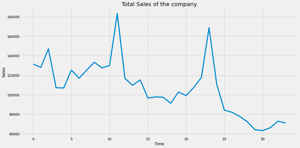
we take total number of items sold in a particular month(we can take the average instead of sum. I tried both but average is unable to give a good result).
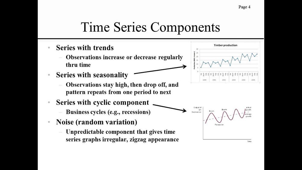
Note: Some distinguishable patterns appear when we plot the data. The time-series has seasonality pattern. Also there seems to be a trend : it seems to go slightly up then down. In other words there are trends and seasonal components in the time series.
Removing trend :
one way to think about seasonal components to the time series to your data is to remove the trend from a time series. So that you can easily investigate seasonality.
Method of removing trend:
- To remove trend, you can subtract the rolling mean from the original signal . This is however will be dependent over how many data points you averaged over.
- Another way to remove trend is method of differencing where you look at the difference between successive data points.
Let’s discuss more about it:
process of rolling average:
here we have to take average of points of either side i.e add the monthly value of the oldest ‘x’ moth period. (x will be an integer)
Note: number of points(x) is specified by a window size which you need to choose.
we are taking average because it tends to smooth out ‘noise’ also.
when it comes to determine the window size, here it makes sense to first try out one of 12 months if you are taking yearly seasonality.
Process of Differencing :
Here we just calculate the difference of successive data points in the time series.
Reason of doing that: it is so much helpful in tuning your time series in a stationary time series.
First order difference:
count= ts[‘count’]
count.diff().plot(figsize=(20,10),linewidth=5,fontsize=20)plt.xlabel(‘time’,fontsize=20)
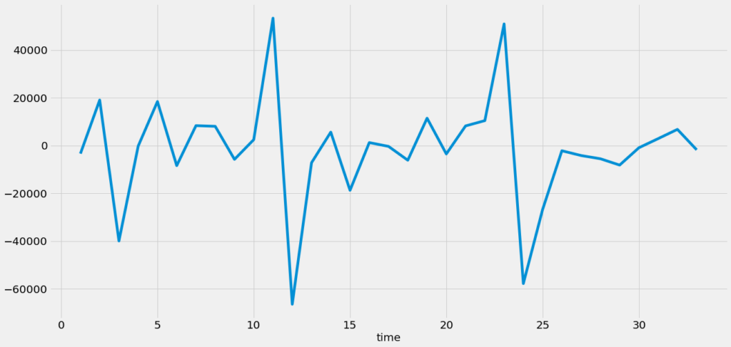
we can see we are able to remove much of the trend & we can really see a good result. If the trend hasn’t removed then we have to look for 2nd order differencing.
Some important concepts:
- STATIONARY TIME SERIES: in simple words a time series is one whose statistical properties (mean & variance) don’t change over time. We need to convert the time series Stationary because forecasting methods(discussed later) are based on the assumptions that time series is actually stationary.
2. Periodicity : A time series is periodic if it repeats itself at equally spaced intervals,say, every 12 months.
3. Autocorrelation: The autocorrelation function is one of the tools used to find patterns in the data. Specifically, the auto correlation function tells you the correlation between points separated by time lags. ACF tells you how correlated points are with each other, based on how many time steps they are separated by.
How to check Stationarity :
- Look at Plot
- Summary Statistics
- Statistical tests
Summary Statistics:
A quick and dirty check to see if your time series is stationary or not ,you can split your time series into two or more partitions and compare mean & variance of each group. If they differ and the difference is significant, the time series is likely to be non stationary.
Augmented Dickey-Fuller test
The Augmented Dickey-Fuller test allows for higher-order autoregressive processes by including Δyt−pΔyt−p in the model. But our test is still if γ=0.
Δyt=α+βt+γyt−1+δ1Δyt−1+δ2Δyt−2+…
The null hypothesis for the test is that the data is non-stationary. We want to REJECT the null hypothesis for this test, so we want a p-value of less that 0.05 (or smaller).
i.e if p- value is >0.05 then differencing is needed to make the process Stationary.
Time series forecasting with ARIMA
We are going to apply one of the most commonly used method for time-series forecasting, known as ARIMA, which stands for Autoregressive Integrated Moving Average.
ARIMA models are denoted with the notation ARIMA(p, d, q). These three parameters account for seasonality, trend, and noise in data.
p: Number of lag observations included in the model.
d: degree of differencing.
q: the order of the moving average
Hey if you want theory and maths behind it please comment down below.
model = ARIMA(ts[‘count’].values, order=(1, 1, 1))
fit_model = model.fit(trend=’c’, full_output=True, disp=True)
fit_model.summary()
Results:
| Dep. Variable: | D.y | No. Observations: | 33 |
|---|---|---|---|
| Model: | ARIMA(1, 1, 1) | Log Likelihood | -373.574 |
| Method: | css-mle | S.D. of innovations | 19171.546 |
| Date: | Mon, 13 Jul 2020 | AIC | 755.147 |
| Time: | 11:58:15 | BIC | 761.133 |
| Sample: | 1 | HQIC | 757.161 |
| coef | std err | z | P>|z| | [0.025 | 0.975] | |
|---|---|---|---|---|---|---|
| const | -1930.2075 | 547.470 | -3.526 | 0.001 | -3003.228 | -857.187 |
| ar.L1.D.y | 0.4257 | 0.163 | 2.616 | 0.014 | 0.107 | 0.745 |
| ma.L1.D.y | -1.0000 | 0.090 | -11.110 | 0.000 | -1.176 | -0.824 |
| Real | Imaginary | Modulus | Frequency | |
|---|---|---|---|---|
| AR.1 | 2.3491 | +0.0000j | 2.3491 | 0.0000 |
| MA.1 | 1.0000 | +0.0000j | 1.0000 | 0.0000 |
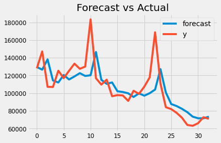
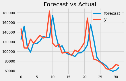
Let’s plot this:
fit_model.plot_predict()
plt.title(‘Forecast vs Actual’)
pd.DataFrame(fit_model.resid).plot()
forcast = fit_model.forecast(steps=6)
pred_y = forcast[0].tolist()
pred = pd.DataFrame(pred_y)
The Akaike information criterion (AIC) is an estimator of out-of-sample prediction error and thereby relative quality of statistical models for a given set of data. Given a collection of models for the data, AIC estimates the quality of each model, relative to each of the other models.
Here the AIC is 755.147. I am happy with that results. Hey do we need 2nd order differencing?(d=2)
ans: No from my side. But let’s try.
model = ARIMA(ts[‘count’].values, order=(1, 2, 1))
fit_model = model.fit(trend=’c’, full_output=True, disp=True)
fit_model.summary()
Results:
| Dep. Variable: | D2.y | No. Observations: | 32 |
|---|---|---|---|
| Model: | ARIMA(1, 2, 1) | Log Likelihood | -367.756 |
| Method: | css-mle | S.D. of innovations | 22262.760 |
| Date: | Mon, 13 Jul 2020 | AIC | 743.512 |
| Time: | 11:58:21 | BIC | 749.375 |
| Sample: | 2 | HQIC | 745.456 |
| coef | std err | z | P>|z| | [0.025 | 0.975] | |
|---|---|---|---|---|---|---|
| const | -73.2828 | 329.027 | -0.223 | 0.825 | -718.165 | 571.599 |
| ar.L1.D2.y | -0.2607 | 0.168 | -1.552 | 0.131 | -0.590 | 0.068 |
| ma.L1.D2.y | -1.0000 | 0.084 | -11.969 | 0.000 | -1.164 | -0.836 |
| Real | Imaginary | Modulus | Frequency | |
|---|---|---|---|---|
| AR.1 | -3.8366 | +0.0000j | 3.8366 | 0.5000 |
| MA.1 | 1.0000 | +0.0000j | 1.0000 | 0.0000 |
Hmmmmm….!
Lower the AIC better will be the result. But the AIC doesn’t change that much. So it’s not needed.
plot this:
Summary:
specially you have learned:
- The importance of time series data being stationary for use & how to check stationarity in a time series data.
- How to do forecasting with Arima.
3. How to eliminate trend by the method of differencing.
In the next part of the tutorial we will discuss a little bit about this result and the results with PROPHET and NEURAL NETWORKS.
Thank You
part 2:
[likebtn counter_type=”percent” bp_notify=”0″]

i like this fabulous post
Hi Mr Souvik Manna. Amazing post!
Can I please have your email address? I could really benefit from your knowledge on Time Series.
Hello Jonitha,
You can mail us on [email protected].