Discrete probability Distributions

In this article we will touch upon the major discrete distributions briefly.

1. Bernoullian Distribution:
   

A trial is said to be bernoullian trial if:

1. the trials have only 2 outcomes. (namely success and failure)
   
2. Outcomes are independent of each other.
   
3. Probability of occurring of any trial remains same in each trial.
   

Let us define a Random variable X such that it has only two outcomes success(S) and failure(F). Then the probability distribution of X is given by:

Where p is the probability of occurrence of success. Then we denote it as,

X ~ ber (p)

The P.M.F (Probability Mass function) of X is:

f(x) = p^x (1-p)^(1-x) for x = 0,1

Mean:

Variance: Var(x) = p(1-p)

Example: Let us consider a trial of coin tossing. We call the occurrence of head as a success (1) and the occurrence of tail as a failure (0). Then this trial follows a Bernoulli distribution with p=0.5.

Few other models following Bernoulli distribution are:

• A new born child is either male or female. (Here the probability of a child being a male is roughly 0.5.)
  

• You either pass or fail an exam.
  
• A tennis player either wins or loses a match. (p=0.5)
  

The PMF must be intuitive to you. It is just a special case of binomial distribution where number of trials is 1.

Application of Bernoulli trial in R-software.

## In R there is no inbuilt code for Bernoulli trial. So we use the inbuilt code of binomial distribution by setting the value of parameter n as 1.

## Suppose we have a unbiased coin with probability of head = 0.7. We call the occurrence of head as success (1)

## suppose we want to make ten simulations using the above information

Code-

n=1

p=0.7

rbinom(10, n, p)

Output-

1 1 0 1 1 1 1 0 1 1

## the R code has given us ten simulations on the basis of Bernoulli distribution and its specified parameters.

# 1 indicates head and 0 indicates tail

## PDF of the distribution

Code –

dbinom(1,n,p)

## 1 indicates success which we have specified as getting head. The above code will give us the probability of getting a head which we have specified as 0.7. Suppose we put 0 instead of 1, it will give us the probability of getting a tail which is 0.3

r- Simulations from the distribution.

d- PMF from the distribution.

q- Percentiles of the distribution.

p- CMF (cumulative mass function) of the distribution.

The codes qbinom and pbinom will give us the quantile and CMF of the distribution respectively.

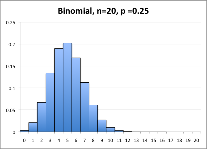
1. Binomial Distribution:
   

When we perform ‘n’ Bernoulli trials with success probability ‘p’ and we count the number of success out of these ‘n’ trials, then the Random variable denoting this number of success is called Binomial Random variable.

Let X denote the number of success with success probability ‘p’. Then we denote it as:

X ~ Bin (n, p)

The P.M.F (Probability Mass function) of X is:

for x = 0,1,2……..,n

Mean:

Variance: Var(x) = n*p*(1-p)

Example: Let we are tossing 10 coins. The random variable denoting the total number of heads in the 10 Bernoulli trials will follow binomial distribution with pmf:

for x = 0,1,2……10

This denotes the probability of getting ‘x’ number of heads.

In the same way few other models are:

• Rolling a die n number of times. (the number of six occurring in the n trials follows a binomial distribution)
  
• Picking a card from a deck of cards n number of times. (the number of kings drawn follows a binomial distribution)
  
• The number of Alto parked in a parking lot which has a capacity for n car-parkings follow a Binomial distribution with parameter p=0.5.
  

The PMF of the binomial distribution is very intuitive as well.

Application of Binomial distribution in R-Language:

## Suppose we have tossed 10 coins. Each coin is statistically independent and identical to each other. The coins are unbiased with probability of head = 0.7

Code-

n=10

p=0.7

qbinom(0.9, n, p) ## this code will give us the value of number of heads which is at the 90^th percentile of the distribution.

Similarly we can take out PMF & CMF of the distribution using the code dbinom and pbinom respectively.

1. Poison Distribution:
   

If a Bernoulli trial is repeated for large number of times (i.e. for large n), with very small success probability ‘p’ such that n*p is finite constant then the number of success for large number of Bernoulli trials follows a Poisson distribution.

The PMF of the poison distribution is a special case of binomial.

The PMF of any discrete distribution such as bernoulli, uniform, binomial, negative binomial distribution is quite intuitive. But same is not the case with poisson distribution. The Poisson(lamda) distribution is a special case of binomial(N, P) distribution. As N becomes large and tend to infinity and P tends to zero, such that the mean N*P remains constant, the binomial distribution leads to the distribution of poisson with parameter – ‘lamda’, which is the average/expected number of success per time period. N*p also gives us the expected number of success. So lamda = N*P, or P = lamda /N. Example– Suppose N =100 and lamda =10, then P =0.1 P(X =10), using binomial is 0.132 and using poisson distribution is 0.12511. When N becomes large to 1000 and the mean is constant at 10, the P is 0.001. P(X=10) using poisson is 0.12511 and using binomial is 0.12574 Similarly, when N =10000, P =0.0001, P(X =10) using binomial is 0.125172. So we can see that as the number of trials, N, becomes too large and tends to infinity and the chance of the occurrence of the event becomes rare and rare which is P tend to zero, the binomial distribution converges to poisson.

A random variable X is said to follow a Poisson Distribution. Then we denote it as:

X ~ Poi(λ)

The P.M.F (Probability Mass function) of X is:

λ>0 x=0,1,2,3………

The most important property of Poisson distribution is that Poisson distribution is a limiting form of binomial distribution. For the following conditions binomial distribution tends to Poisson distribution:

1. n is large.
   
2. P is very small (i.e. the probability of occurrence of a event is very small)
   
3. np= λ is a finite constant.
   

Mean:

Variance: Var(x) = λ

A few examples of Poisson Distribution are:

• Number of Suicides reported in a particular area.
  
• Number of air accidents within some interval of time.
  
• Number of printing mistakes in each page of a book.
  

Application of poison distribution in R – software

## suppose we know that the number of suicides each year in a particular region follows poison distribution with average 10/ year.

Code-

lamda=10

rpois(10,lamda)## this code will simulate 10 values from poison(10) distribution. The each simulation will indicate the number of yearly suicide in the region.

dpois(10,lamda) ## it will give us the probability of observing exactly 10 deaths in the region in a year.

Similarly the codes qpois and ppois will give us the percentile & CMF respectively.

• Geometric Distribution:
  

The geometric distribution represents the number of failures before you get a success in a series of Bernoulli trials.

A random variable X is said to follow a Geometric Distribution. Then we denote it as:

X ~ Geo (p)

The P.M.F(Probability Mass function) of X is:

f(x) =
(1-p)^(x-1) p x=1,2,3……. (I)

Or,

f(x) = (1-p)^x p x=0,1,2,3……. (II)

By convention model (I) consider as the pdf of Geometric distribution.

Basically, it denotes the probability that x trials are required to get the 1^st success.

Mean:

Variance:

The PMF of this distribution is very intuitive as well.

Examples:

• Suppose balls are drawn from a sack containing white and black balls. The random variable denoting the number of black balls drawn before the 1^st white ball is drawn follows a geometric distribution.
  
• You are planning to go to shopping Mall by Auto-rickshaw. You are asking each and every empty Auto-rickshaw passing by for the ride. To find the probability of getting denied by an auto-rickshaw 1,2,3…. Times before getting a ride, we use Geometric distribution.
  

Application of geometric distribution in R- Language:

## Suppose a couple is planning their future. Now they want to know the probability of getting first baby boy after two baby girls. The probability of getting a boy or girl at any time is same and is independent of each other.

Code:

p=0.5

dgeom(2,p) ## Running this code will give us the required probability which is 0.125

rgeom(10,p) ## this code will generate 10 simulations for us. Each simulation indicates the number of babies after their first baby boy was born.

Similarly the code pgeom and qgeom will give us the CMF and percentiles respectively.

• Negative Binomial Distribution:
  

  The negative binomial distribution denotes the probability of getting the k^th success in x^th trial.
  

If a random variable X is said to follow a Negative Binomial Distribution, then we denote it as:

X ~ NB (k, p)

The P.M.F (Probability Mass function) of X is:

x=0, 1, 2………

Mean:

Variance:

Examples:

• Consider the following statistical experiment. You flip a coin repeatedly and count the number of times the coin lands on heads. You continue flipping the coin and want to the chance that it will land fifth head on ninth trial. This is a negative binomial experiment.
  

Negative Binomial Distribution is the generalized version of Geometric Distribution: In geometric distribution we find the probability of the number of trials before the 1^st success and in negative binomial distribution we find the probability of the number of trials required to get the k^th success.

Interesting Facts: (For identifying a distribution from a given discrete data)

First, we calculate the Mean and variance of the dataset given. Then we check the inequality of the mean and variance.

1. If mean=variance then the data is appropriate for fitting in the Poisson distribution. Since for Poisson distribution mean= and variance =
   
2. If mean>variance then the data is appropriate for fitting in the Binomial distribution. Since for Binomial distribution mean= np and variance = np(1-p)
   

1. If mean<variance then the data is appropriate for fitting in the Negative Binomial distribution. Since for Negative Binomial distribution mean= k/p and variance =