Deep Feature Synthesis / Introduction to Automated Feature Engineering

“Feature engineering is the art part of data science”
— Sergey Yurgenson
In the context of machine learning, a feature can be described as a characteristic, or a set of characteristics, that explains the occurrence of a phenomenon. When these characteristics are converted into some measurable form, they are called features.
What is Feature Engineering?
ans: Feature Engineering can simply be defined as the process of creating new features from the existing features of the data set.
What is Deep Feature Synthesis?
ans : DFS is an algorithm that automatically generates features for relational data sets. In essence, the algorithm follows relationships in the data to a base field, then sequentially applies mathematical functions along that path to create the final feature. By stacking calculations sequentially, we observe that we can define each new features as having a certain depth. Hence, we call the algorithm Deep Feature Synthesis.
In this article, we will try to explain the impact of DFS and try to compare the results with raw features and the new features.
preference: Google colab or Jupyter Notebook

So let’s start.
Data Set Description:
Company wants to automate the loan eligibility process (real time) based on customer detail provided while filling online application form.
These details are Gender, Marital Status, Education, Number of Dependents, Income, Loan Amount, Credit History and others.
here the dependent column explain the loan status of the customer(Y/N).
Link of the data set is given below:
Importing the necessary packages and the data set:
The dataset has 13 features and 614 rows. We don’t wanna delete any row from the data i.e we don’t wanna loose any information regarding customer’s account details and income.
Data types:
Loan_ID               object
Gender                object
Married               object
Dependents            object
Education             object
Self_Employed         object
ApplicantIncome        int64
CoapplicantIncome    float64
LoanAmount           float64
Loan_Amount_Term     float64
Credit_History       float64
Property_Area         object
Loan_Status           object
dtype: object
Pre-processing Steps:
- Encode the categorical variable
from sklearn.preprocessing import LabelEncoder
LabelEncoder_Y= LabelEncoder()
for column in df.columns:
  if df[column].dtype == np.number:
    continue
  else:
    df[column]=LabelEncoder().fit_transform(df[column])
or simply run this:
from sklearn.preprocessing import LabelEncoder
labelencoder_y=LabelEncoder()
df['Loan_Status']=labelencoder_y.fit_transform(df['Loan_Status'].values)
df['Education']=labelencoder_y.fit_transform(df['Education'].values)
df['Property_Area']=labelencoder_y.fit_transform(df['Property_Area'].values)
2. Missing Values:
sns.heatmap(df.isnull(),cbar=False)
df.isna().sum()

df['LoanAmount']=df['LoanAmount'].replace(np.nan,np.mean(df['LoanAmount']))
df['Loan_Amount_Term']=df['Loan_Amount_Term'].replace(np.nan,np.mean(df['Loan_Amount_Term']))
df['Credit_History']=df['Credit_History'].replace(np.nan,0)
3. Delete those columns we don’t need
[8]:df=df.drop(columns=['Self_Employed','Gender','Married','Dependents'],axis=1)
Now it’s time to build some machine learning model and calculate our first prediction:

The underlying problem we are going to solve comes under the Supervised Machine Learning category. So, let us have a brief discussion about this topic before moving on to apply different Machine Learning models on our dataset.
Supervised Machine Learning :-
The majority of practical machine learning uses supervised learning.
Supervised learning is where you have input variables (x) and an output variable (Y) and you use an algorithm to learn the mapping function from the input to the output.
Y = f(X)
The goal is to approximate the mapping function so well that when you have new input data (x) that you can predict the output variables (Y) for that data.
Supervised learning problems can be further grouped into regression and classification problems.
- Classification: A classification problem is when the output variable is a category, such as “red” or “blue” or “disease” and “no disease” or in our case “Positive” or “Negative”
- Regression: A regression problem is when the output variable is a real value, such as “dollars” or “weight”.
Our problem comes under the classification category because we have to classify our results into either Positive or Negative class.
Here we have used Logistic Regression for comparison purpose.
steps:
- Y is our dependent variable and the other independent variables are chosen as X
- Split the data into test and train
- Scale the data using StandardScaler
X=df.drop(columns=['Loan_ID','Loan_Status'],axis=1)
Y=df['Loan_Status']
X_train,X_test,Y_train,Y_test=train_test_split(X,Y,test_size=0.2,random_state=0)

sc=StandardScaler() X_train=sc.fit_transform(X_train) X_test=sc.fit_transform(X_test)
If you are interested more about logistic regression then check out the link:
from sklearn.linear_model import LogisticRegression
lreg=LogisticRegression()
lreg.fit(X_train,Y_train)predictions=lreg.predict(X_test)
Now after doing prediction we will print our accuracy score and f1_score for further comparison purpose.
print(accuracy_score(predictions,Y_test))
print(f1_score(predictions,Y_test))acuuracy score:0.7886178861788617
f1_score: 0.8617021276595744
Why are we using f1_score and accuracy score?
- it will be explained later. keep reading.
OK it’s time to jump into the automated feature engineering task.
Before that let’s go through some short note and some questions.
What is Featuretools?
Ans: Featuretools is a framework to perform automated feature engineering. It excels at transforming temporal and relational datasets into feature matrices for machine learning.

What is Entity?
Ans : An entity is simply a table or in pandas, a data frame. An entity in featuretools must have a unique index where none of the elements are duplicated.
What is Entity Set?
Ans : An entity set is a collection of tables and relationships between them.This can be thought as a data structure with own methods and attributes. For each relationship we need to specify the parent variable and the child variable.
What are the primitives?
Ans : A feature primitive is an operation applied to a table or a set of tables to create a feature.
Feature primitives are of two types: Aggregation , Transformation
Feature Engineering using Featuretools
Now we can start using Featuretools to perform automated feature engineering! It is necessary to have a unique identifier feature in the data set (loan_id). we have an id but if you don’t have unique id then it will be created. Suppose you have two different ids for two different data sets and you want a unique id then simply concentrating both will solve your problem.
Now it’s time to create our entity set step by step.
Step 1:
- create and entity set is es
- adding a dataframe
es=ft.EntitySet(id='loan')
es= es.entity_from_dataframe(entity_id = 'customer', dataframe =X2, index ='Loan_ID')
Step 2:
We have created a new table from the customer table based on the Loan id.
es = es.normalize_entity(base_entity_id='customer', new_entity_id='LoanAmount', index='LoanAmount')
es = es.normalize_entity(base_entity_id='customer', new_entity_id='ApplicantIncome', index='ApplicantIncome')
es = es.normalize_entity(base_entity_id='customer', new_entity_id='CoapplicantIncome', index='CoapplicantIncome')
es = es.normalize_entity(base_entity_id='customer', new_entity_id='Loan_Amount_Term', index='Loan_Amount_Term')
Step 3:
let’s check summary of our entity set.
> print(es)
Entityset: loan
  Entities:
    customer [Rows: 614, Columns: 8]    LoanAmount [Rows: 204, Columns: 1]    ApplicantIncome [Rows: 505, Columns: 1]    CoapplicantIncome [Rows: 287, Columns: 1]    Loan_Amount_Term [Rows: 11, Columns: 1]  Relationships:
    customer.LoanAmount -> LoanAmount.LoanAmount
    customer.ApplicantIncome -> ApplicantIncome.ApplicantIncome
    customer.CoapplicantIncome -> CoapplicantIncome.CoapplicantIncome
    customer.Loan_Amount_Term -> Loan_Amount_Term.Loan_Amount_Term
Step 4:
Now we will use Deep Feature Synthesis to create new features automatically. Recall that DFS uses Feature Primitives to create features using multiple tables present in the EntitySet.
default_agg_primitives =  ["sum", "max", "min", "mean", "count"]

# DFS with specified primitive
feature_names = ft.dfs(entityset = es, target_entity = 'customer',
                       agg_primitives=default_agg_primitives,
                       max_depth = 2, features_only=True)

print('%d Total Features' % len(feature_names))
So it is giving 59 Total Features.
feature_matrix, feature_names = ft.dfs(entityset = es, target_entity = 'customer',
                                       agg_primitives=default_agg_primitives,
                                        max_depth = 2, features_only=False, verbose = True)

pd.options.display.max_columns = 1700
feature_matrix.head(10)
Bingo! We have created new features based on the existing data set.
Note: Yeah that sounds great that we have created a lot of features but we are going to face a serious problem of over fitting. So we should keep it in mind.
Step 5:
in case if you want to store it in your computer. Just run the following code:
>feature_matrix = feature_matrix.reset_index()
>print(‘Saving features’)
>feature_matrix.to_csv(‘new_df.csv’, index = False)
Now we have completed most of the job. It’s time to see how our logistic regression works for our new data frame.
Before that calculate the correlation among features and delete those features which are highly correlated . It will reduce the power of over fitting.
Featuretools Interpret-ability
Making our data science solutions interpretable is a very important aspect of performing machine learning. Features generated by Featuretools can be easily explained even to a non-technical person because they are based on the primitives, which are easy to understand.
For example, the features ApplicantIncome.SUM(customer.Credit_History)and ApplicantIncome.MEAN(customer.Credit_History)mean applicant’s sum and mean of credit history respectively.
This makes it possible for those people who are not machine learning experts, to contribute as well in terms of their domain expertise.

X3= new_df
X_new=X3.drop(columns=['Loan_ID'],axis=1)

corr=X_new.corr().abs()upper=corr.where(np.triu(np.ones(corr.shape),k=1).astype(np.bool))
threshold=0.7
collinear_features=[column for column in upper.columns if any(upper[column]>threshold)]
Note : here we have used a threshold of 0.7. You can use whatever you want according to your problem.
X=X_new.drop(X_new[collinear_features],axis=1)

Model Building:
splitting:
X_train,X_test,Y_train,Y_test=train_test_split(X,Y,test_size=0.2,random_state=0)
scaling:
X_train=sc.fit_transform(X_train)
X_test=sc.fit_transform(X_test)
# logistic regression
from sklearn.linear_model import LogisticRegression
lreg=LogisticRegression()
lreg.fit(X_train,Y_train)
>LogisticRegression(C=1.0, class_weight=None, dual=False, fit_intercept=True,
intercept_scaling=1, l1_ratio=None, max_iter=100,
multi_class=’auto’, n_jobs=None, penalty=’l2′,
random_state=None, solver=’lbfgs’, tol=0.0001, verbose=0,
warm_start=False)
predictions2=lreg.predict(X_test)
f1_sore:
f1_score(predictions2,Y_test)
Output:
0.870967741935484
Accuracy score:
accuracy_score(predictions2,Y_test)
Output:
0.8048780487804879
Hurrah! we are done.
Comparison:
previously the accuracy score was 0.78(approx) and now it has reached to 0.8.
previously f1_score was 0.8617021276595744 and now it’s 0.870967741935484.
We can do more better if we use some ensemble techniques or if we use different threshold. Please let me know if you get some better results. I hope you will.
Why F1 Score ?
Let us generate a countplot for our training dataset labels i.e. ‘0’ or ‘1’ .
sns.countplot(df['Loan_Status'],label='count')

- From the above countplot generated above we see how imbalanced our dataset is.We can see that the values with label : Y valuesare quite high in number as compared to the values with label : N values..
- So when we keep confusion matrix as our evaluation metric there may be cases where we may encounter high number of false positives. So that is why we use F1 Score .

End Notes:
The featuretools package is truly a game-changer in machine learning. While it’s applications are understandably still limited in industry use cases, it has quickly become ultra popular in hackathons and ML competitions. The amount of time it saves, and the usefulness of feature it generates, has truly won me over.
Happy Reading !!!
I will suggest you to use Xg-boost and see the results. I will explain how xgboost works in such case and why xgboost is more preferable in the next article. Till then follow me and give a clap if you like this.

i love this terrific article
Thanks a lot for providing individuals with an extremely breathtaking opportunity to read critical reviews from this site. It’s usually very awesome and as well , jam-packed with a lot of fun for me and my office acquaintances to visit your website at the very least three times in 7 days to learn the fresh tips you have got. And of course, I am just actually fulfilled with all the incredible suggestions you give. Selected two facts on this page are absolutely the simplest we have had.
I would like to show my thanks to you for bailing me out of such a instance. As a result of exploring throughout the the net and getting thoughts which were not pleasant, I believed my life was well over. Living minus the strategies to the issues you have resolved all through your entire posting is a critical case, as well as those which might have in a wrong way damaged my career if I hadn’t discovered your web page. Your own personal talents and kindness in handling every part was very helpful. I’m not sure what I would’ve done if I had not come upon such a solution like this. I can also now look ahead to my future. Thank you very much for your specialized and amazing help. I won’t think twice to recommend your web site to any individual who needs assistance about this situation.
I simply had to appreciate you once again. I do not know what I would’ve gone through without the strategies shown by you on such theme. It previously was a very intimidating scenario in my view, however , witnessing the very skilled way you treated the issue forced me to cry over fulfillment. Extremely thankful for your information as well as have high hopes you really know what a great job you are always providing training many people through your webblog. I’m certain you haven’t come across any of us.