Analysis of Variance One-Way:

The total variation present in a set of observable quantities may under certain circumstances be partitioned into a number of disjoint components associated with the nature of classification of the data. This systematic methodology by which one can partition the causes of variation into several components is called analysis of variance.
Let us consider an example of yield of paddy. Suppose the yield is carried out using three kinds of seeds. So, the yield variation occurs due to variation of seed and also due to some random error (the position of seed was suitable for germination). This is a classic example of one-way layout of ANOVA.
Assumptions:
- The observations recorded were independent
- Parent population from which observations were taken have normal distribution.
- Homogeneity of variances in the different treatment groups i.e. the variance of all the treatment groups are equal.
One Way ANOVA:
The main theory behind CRD is One-way ANOVA.
Let us consider the following Example.
A spots analyst wanted to know if the physical weight of players differs due to different training strategy of 5 different clubs. For this purpose, he gathered 5 groups from each of the 5 clubs.
Theory:
Here Weight of a player is influenced by a single treatments/Factor, Club, A and the factor has 5 levels.
A (Factor): Clubs from which a professional football player plays for.
Level 1 (Cowboys): players from the Dallas Cowboys
Level 2 (Packers): players from the Green Bay Packers
Level 3 (Broncos): players from the Denver Broncos
Level 4 (Dolphins): players from the Miami Dolphins
Level 5 (Niners): players from the San Francisco Forty Niners
So, there are 5 treatments and ith treatment (where i=1, 2, 3, 4, 5) is replicated ri =17 times. i.e., it can look upon as a similar setup like ANOVA one may fixed effect model, where a single factor has 5-levels and each level consists of ri =17
observations.
For ith level, let there be ni observations,

We represent the observations in the following array data.


One-way fixed effect model is given by:

yij = response corresponding to jth observation of ith level of A
µi = effect due to ith level of A.


αi = additional effect due to i-th level of A
µ= general effect
eij = error in model
Re-parameterization essentially leads to separation of error and exact effect due the factor A
Generally, the two hypotheses are considered as:
H0: α1 = α2 = α3= α4= α5 v/s H1: at least one inequality
The following two hypotheses can be described as:
H0: there is no difference between mean weights of players from different clubs
Vs.
H1: at least one of the mean weights is different from another
One -way ANOVA using R:
Code:
[Note:
Do not choose Excel formal for this case as it doesn’t read the levels of a factor
Consider the following code and output for illustration:
> player_weight <- read_excel(“E:/mathematicacity/player weight.xlsx”,
+ col_types = c(“numeric”, “text”))
> View(player_weight)
> names(player_weight)
[1] “Weight” “Club”
> levels(player_weight$Club)
NULL
Note that R cannot read its levels. (Giving output as NULL)]
#Choosing dataset (if the dataset is in .csv Format)my_data <- read.csv(file.choose())View(my_data)
Preview of the data:
|
Weight |
Club |
|
250 |
Cowboys |
|
255 |
Cowboys |
|
255 |
Cowboys |
|
264 |
Cowboys |
|
250 |
Cowboys |
|
265 |
Cowboys |
71 more columns
# Show the levelsnames(my_data)levels(my_data$Club)
Output:
[1] "Weight" "Club"
[1] "Broncos"  "Cowboys"  "Dolphins" "Niners"
[5] "Packers"
#Estimation of Modelmodel1 <- aov(Weight ~ Club, data = my_data)summary(model1)
| Df | Sum sq. | Mean Sq. | F value | Pr(>F) | |
| Club | 4 | 1714 | 428.4 | 1.575 | 0.189 |
| Residuals | 80 | 21761 | 272.0 |
Signif. codes: 0 '***' 0.001 '**' 0.01 '*' 0.05 '.' 0.1 ' ' 1
The output includes the columns F value and Pr(>F) corresponding to the p-value of the test. From the p-value we cannot reject the Null Hypothesis at 5% level of Significance.
So, we can conclude that at 5% level of Significance the physical weight of plyers does not differ significantly due to different training strategy of 5 different clubs.
[Note:
But if the Null hypothesis was rejected then we can perform a paired comparison with the help of Tukey test and can find out which club’s training strategy differs significantly. The R code for this is:
TukeyHSD(model1, conf.level = 0.95)
We will consider an example in the Next portion of 2-way ANOVA so that we can perform the Tukey test.]
##Checking ANOVA assumptions# 1. Homogenity of variancesinstall.packages("car")library(car)leveneTest(Weight ~ Club, data = my_data)
Output:
Levene's Test for Homogeneity of Variance (center = median)
      Df F value Pr(>F)
group  4  0.0956 0.9836
      80
From the output above we can see that the p-value is not less than the significance level of 0.05. This means that there is no evidence to suggest that the variance across groups is statistically significantly different. Therefore, we can assume the homogeneity of variances in the different treatment groups.
# 2. Normalityplot(model1, 2)# Extract the residualsaov_residuals <- resid(model1 )# Run Shapiro-Wilk testshapiro.test(x = aov_residuals )
Output:

Shapiro-Wilk normality test
data:  aov_residuals
W = 0.94462, p-value = 0.001161
From the p-value and the plot we can see that the data does not violate the Normality assumption.

I needed to draft you this bit of remark just to say thanks the moment again on your superb suggestions you’ve shown on this website. It is really surprisingly generous with you giving openly precisely what a number of people would have offered for an ebook to earn some dough for their own end, most notably considering that you could have tried it if you ever considered necessary. The tricks as well worked as a good way to understand that other people online have the identical passion similar to mine to see a whole lot more with reference to this matter. Certainly there are lots of more pleasant sessions ahead for people who read through your website.
I wish to show some thanks to you just for bailing me out of this type of instance. After looking throughout the world-wide-web and meeting concepts which are not pleasant, I was thinking my life was well over. Being alive without the presence of solutions to the difficulties you have fixed through the posting is a crucial case, as well as those which may have negatively damaged my career if I hadn’t noticed your web page. That competence and kindness in taking care of all the details was precious. I am not sure what I would have done if I hadn’t encountered such a step like this. I am able to now look forward to my future. Thank you very much for this high quality and results-oriented guide. I won’t hesitate to refer your web blog to anybody who wants and needs guide about this area.
I must show my appreciation for your kind-heartedness giving support to people who really want guidance on the niche. Your real commitment to getting the solution up and down appeared to be amazingly productive and has consistently encouraged employees like me to get to their aims. This insightful help indicates a whole lot to me and extremely more to my office colleagues. Regards; from everyone of us.