Simple Linear Regression

Theory

The simple linear regression model is used when there are only two variables and there exists a linear relationship between the two variables of the form-

Ŷ= a + b*X

Ŷ is the predicted value of the variable Y. It is the response or dependent variable.

X is the independent variable.

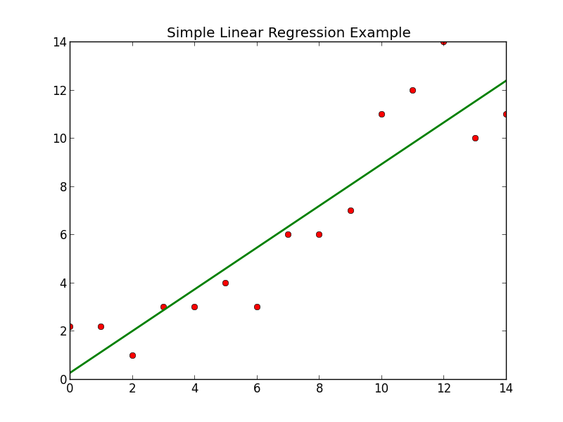
The “a” is the Y- intercept. It is the value of Y when the value of X is zero. In the above diagram we can see that when X is zero, the value of Y is 6. Hence, in the above diagram, “a” is 6.

The “b” is the slope of the line. It tells us the change in the value of Y with the change in the value of X.

The difference between the actual and estimated value of Y is termed as residuals. It is the part that is not explained by the model. Residuals are also known as error terms and denoted by “e”.

Residual = e=Y- Ŷ = actual value – value estimated using the model.

The values of a and b are estimated using method of least square-

Q= ∑e^2 = ∑(Y-Ŷ) ^2

      =∑(Y-(a + b*X)) ^2

Now, our model will be good if the value of Q is as small as possible and close to zero.

So we will have to find the value of a and b such that the function Q is minimised.

This can be easily done by partially differentiating the function with respect to a and b. I am leaving the derivation part on readers. This is how the value of a and b can be found.

By double differentiation, one can check if the values of a and b are minimising the function.

Now the value(s) of Y can be estimated for the given value(s) of X.

The actual value of Y will be = a + b*X + residual.

The residuals are assumed to be normally distributed with mean zero and variance sigma^2.

The closer the correlation is to 1 in absolute terms, the better the predictions will be and the stronger will be the linear relationship between the two variables.

             SIMPLE LINEAR REGRESSION USING R SOFTWARE

Suppose we are to predict annual inflation index. Now, we know the inflation index increases with time. We can check this by seeing the correlation between the two. The closer the correlation is to 1, the stronger is the positive linear correlation between the two variables.

Steps for linear prediction in R software:

Step 1

First of all import the data to your R. Suppose the data is in D drive of your computer with the name “index” in “csv” format. You can check the format of the data by clicking on the properties and you can also change it according to you.

setwd("D:\\")##this code will tell R in which directory your data is stored in                                                                                                              your computer.
a= read.csv(“index.csv”, header = T)##this will enable R to read the data “index” which is in“csv” format in your computer. The data is stored in the variable “a” here. The data has header as “year” and “index” so I have given header = T.

Step 2

Check for linearity between year and index. If there exists a strong linear relationship between the two, then only we will be able to use simple linear model for predictions.

This can be tested by scatter plot.

plot(a$year, a$index) ##this will give us the scatter plot with year on the x-axis and indexes on the y-axis.The output of the code is given below: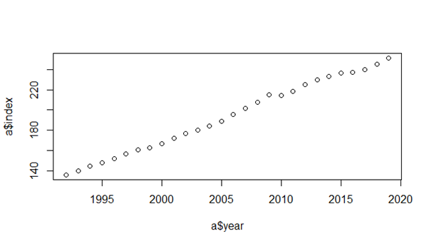

We can clearly see that there is no outlier and the relationship is strongly linear.

cor(a$year, a$index) ##this code will tell you the correlation between the year and inflation index.

The closer is the correlation to the absolute value of 1, the stronger is the linear relationship between the two variables.

Step 3

Here we will be predicting the indexes using simple linear model.  The index will be our dependent variable and year will be our independent variable.

lm(a$index ~ a$year) ## this code will give us the value of y-intercept and slope of the line when index is dependent on year.

In Y= a+b*X, the code will give us the value of a and b. Below is the output of the code.

                           Coefficients:
                      (Intercept)       a$year  
                        -8551.20         4.36

predict(lm(a$index~a$year))##this code will give us the predicted value of indexes for all the given years in our data.
NOTE- both year and index must contain equal number of data for this code to run. 

Step 4

Now we need to check how well the predictions or the simple linear model fits the actual data

Just one code will tell us the entire summary of our fit. Understanding the output here is more important than writing the code.

summary(lm(a$index~a$year)) ## this code will tell us the entire summary about the fitted      model and how good is the fit. 

                      Residuals:
               Min     1Q   Median     3Q     Max 
             -3.717 -2.265   0.313   1.480   6.461 

Coefficients:
            Estimate   Std. Error  t value  Pr(>|t|)    
(Intercept) -8551       116.455    -73.43   <2e-16 ***
a$year       4.36       0.05807     75.09   <2e-16 ***
---
Signif. codes:  0 ‘***’ 0.001 ‘**’ 0.01 ‘*’ 0.05 ‘.’ 0.1 ‘ ’ 1

Residual standard error: 2.482 on 26 degrees of freedom
Multiple R-squared:  0.9954,	Adjusted R-squared:  0.9952 
F-statistic:  5639 on 1 and 26 DF, p-value: < 2.2e-16

Understanding the output:

Residual are the part unexplained by the model. The smaller it is, the better is our model. We assume the residuals to follow normal distribution with mean zero and variance sigma^2, so the median of the residuals must be close to zero.

Coefficients– t-value = (coefficient estimate) / (standard error)

The higher the t-value, more significant is the coefficient.

The coefficient “b” of year has estimate of 4.36. It means that index increases by 4.36 for every year.

Under null hypothesis, b = zero and we have got b= 4.36 just by chance due to the sample used.

The t-value is -73.43 which is significantly high and the probability of getting this value of t by chance when b is zero is very close to zero (see the adjacent column of the output).

Since it less than 5% (our favourite choice), we reject null hypothesis with sufficient evidence at 5% L.O.S

The asterisk beside the coefficients tells us about their significance. We can remove the ones with no significance or little significance from our model. This is very useful in multi-linear regression model fitting. Three asterisks shows very high significance.

Residual standard error– it tells us how far the actual data are from their predicted value on an average. The less it is, the better is our model.

R–squared= (Sum of square of regression) ÷ (sum of square of total)

                                            = ((Y^ – Y̅̅̅) ^2) ÷ ((Y- Y̅) ^2)     

Y̅ is the mean of independent variable Y.

It tells us the proportion of variation in Y explained by the proportion of variation in X. The closer it is to one, the better is our model.

The adjusted R-squared is of use in multi-linear regression which will be explained by us in the next article. It is of no use in simple linear model.Note– inflation index depends on lot of other factors as well such as GDP, employment rate etc. You can easily get the data of indexes from the internet. In the next article we will post about multi-linear regression model.

Kounteyo Roy Chowdhury

Msc in applied statistics.
Data Scientist specializing in AI-NLP

LinkedIn